"2D Fokker-Planck models of rotating clusters" |
|---|
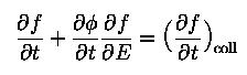
 and
and

 were used)
 , σc: central velocity dispersion
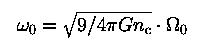 ,dimensionless angular velocity (rotating parameter)
 ,dimensionless potential (King parameter)
The dynamical ellipticity is calculated following Goodman (1983), given by
Initial parameters of the 12 rotating cluster models.
| King parameter Wo | rotating parameter ωo | |||||
|---|---|---|---|---|---|---|
| 3.0 | 0.0 | 0.30 | 0.60 | 0.90 | ||
| 6.0 | 0.0 | 0.30 | 0.60 | 0.90 | ||
| 9.0 | 0.0 | 0.06 | 0.08 | 0.10 | ||
Evolution grid in interval coordinates for the 12 models. The cells contain the total number of datasets available for the grid point with given time and ellipticity.
| Ellipticity | Time (t/trh) | |||||
|---|---|---|---|---|---|---|
| (0,2) | (2,4) | (4,6) | (6,8) | (8,10) | (10,12) | |
| (0.00-0.02) | 59 | 16 | 40 | 93 | 58 | 58 |
| (0.02-0.04) | 5 | 24 | 15 | 10 | ||
| (0.04-0.06) | 8 | 27 | 9 | 14 | ||
| (0.06-0.10) | 28 | 62 | 11 | 2 | ||
| (0.10-0.15) | 19 | 24 | 3 | |||
| (0.15-0.20) | 6 | 7 | ||||
| (0.20-0.25) | 4 | |||||
| (0.25-0.30) | 5 | |||||
| (0.30-0.50) | 3 | |||||
We present the evolution in time of global parameters, classified by initial King- and rotating parameters (see description below)
| Model (Wo, ωo) | Datafiles |
|---|---|
| (3,0.00) | time030_000 |
| (3,0.30) | time030_030 |
| (3,0.60) | time030_060 |
| (3,0.90) | time030_090 |
| (6,0.00) | time060_000 |
| (6,0.30) | time060_030 |
| (6,0.60) | time060_060 |
| (6,0.90) | time060_090 |
| (9,0.00) | time090_000 |
| (9,0.06) | time090_006 |
| (9,0.08) | time090_008 |
| (9,0.10) | time090_010 |
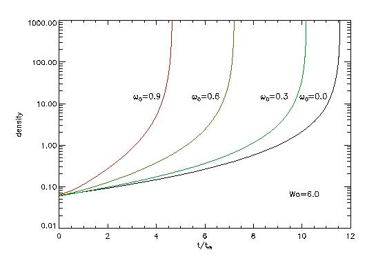
The figure shows the acceleration of core-collapse due to rotation (central density in code units vs. time). The black line represents a non-rotating, the red line a high initial rotating case (ωo=0.9). See also Fig. 3 of Fiestas et al. 2004.
![]() -routine to generate the plot: dtime.pro
-routine to generate the plot: dtime.pro
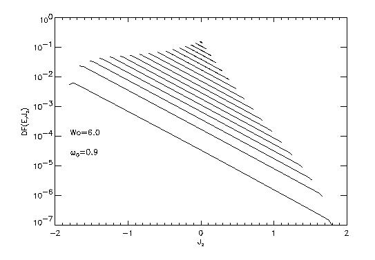
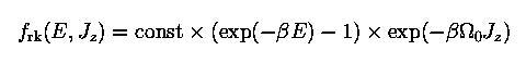
The figure shows the initial distribution function (King model) against angular momentum (curves of constant energy) for the model (6.0,0.3) See also Figs. 1 and 2 of Fiestas et al. 2004.
![]() -routine to generate the plot: df.pro
-routine to generate the plot: df.pro
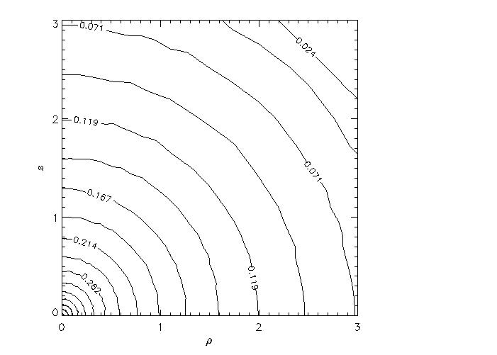
The figure shows a contour map (on meridional plane) of the rotational velocity for a collapsed model of initial (6.0,0.9) at time t/trh=4.7. Distances are given in units of initial core radius, velocity in code units.
![]() -routine to generate the plot: vrot.pro
-routine to generate the plot: vrot.pro
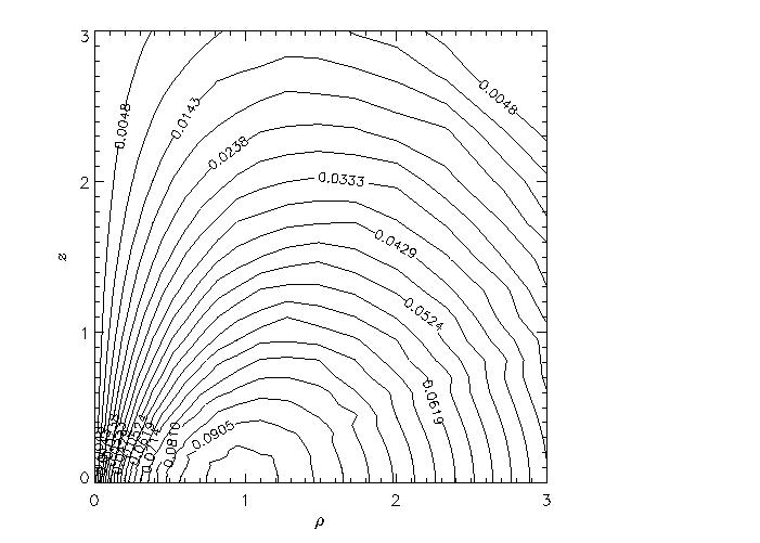
Contour map of 1-d velocity dispersion (on meridional plane) for a collapsed model of initial (6.0,0.9) at time t/trh=4.7. Distances are given in units of initial core radius, velocity in code units.
![]() -routine to generate the plot: vdisp.pro
-routine to generate the plot: vdisp.pro
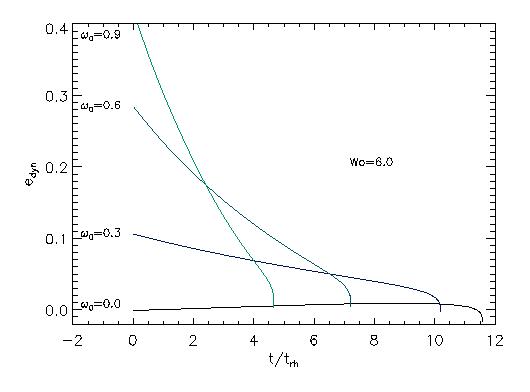
This figure shows the time evolution of dynamical ellipticity for the model Wo=6 and different initial rotation parameters (See also Fig. 4 of Fiestas et al. 2004).
![]() -routine to generate the plot: edynage.pro
-routine to generate the plot: edynage.pro
 and set to 1